By Kate Freund, University of Minnesota
As part of the WinterTurf project, we are using LC-MS based metabolomic methods to examine potential biochemical markers of cold tolerance in perennial ryegrass (see Using untargeted metabolomics to assess cold tolerance in perennial ryegrass- Part 1 and the conclusion in Part 2). Large amounts of data are collected in metabolomic experiments and several inspection and processing steps are required prior to statistical analysis. Grass samples are collected and extracted, and spectral data is collected on the chemical features present in the extracts using HPLC-MS. We use the term “features'' to describe signals in the spectral data, instead of metabolite, compound, or molecule, because at this early stage of the analyses we cannot be certain that the signal we are seeing corresponds with an actual molecule or a fragment of a molecule. The total spectral data for each sample run can be thought of as a “snapshot”, as each extract is a profile of the plant’s chemical composition at the particular time of harvest. The feature data is collected by the HPLC-MS in the form of retention time (how long a feature was retained on a chromatography column), the mass/charge ratio (the mass of the feature divided by the charge number), and UV-vis spectroscopic data (the amount of discrete wavelengths absorbed at a particular time). A single sample can yield hundreds to thousands of unique chemical features, some of which might help us better understand turfgrass winter survival; so how do we process and make sense of this enormous data set?
Data visualization
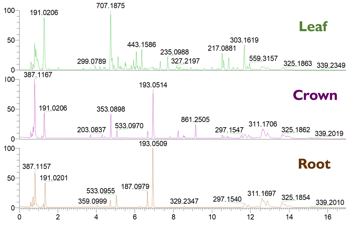
We start with data visualization. Once a sample has been analyzed by the HPLC-MS, the data can be visualized in a chromatogram. A chromatogram is a two-dimensional plot with the x-axis showing retention time and the y-axis showing the abundance of a given signal relative to the most abundant feature. Figure 1 shows a comparison of perennial ryegrass leaf, crown, and root tissue samples run using the same HPLC-MS method, with m/z (mass divided by charge) values listed above specific peaks. We see from this comparison that different tissues from the same plant share some features in common, but each also contain features unique to tissue type. Every peak is a signal or series of signals detected by the mass spectrometer. Prior to exporting and processing the data, the chromatogram from each sample run should be visually inspected to ensure the highest quality data. The ideal chromatographic peaks should be Gaussian (“bell curved”) and resolved (meaning signals for different features are separated from one another).
Data processing
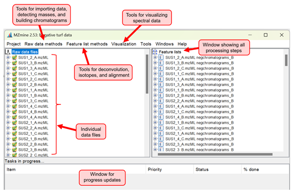
Once we have visualized the data and are confident in our chromatography and mass measurements, we continue on to data processing. Before we can statistically analyze the data, we have to take it through a series of processing steps. The HPLC-MS data is first converted from the .raw file format to .mzml using the ProteoWizard tool msconvert, then imported into MZmine, our preferred open-source software (Figure 2). The HPLC-MS software continuously records masses detected throughout a run, so you can think of this as a list of masses detected at every given time point (or “scan”). A list of masses is generated for each scan, while signals falling under a specified noise level are eliminated. Chromatograms are then built based on these mass lists and additional methods are utilized to reconcile isotopes, align corresponding peaks across different samples, and search for missing peaks. Finally, we manually validate our feature list by inspecting the peaks, making sure they aren’t too broad or undefined.
Statistical analysis
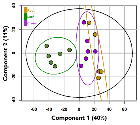
When we are satisfied with the feature list, we export this data as a .csv file and import it into the programming language R for statistical analysis. The series of statistical tests we conduct depends on the design of the original experiment. For targeted metabolomic approaches (see part 1 of previously referenced blog post for an explanation of targeted vs. untargeted), it is appropriate to use univariate analyses such as ANOVA and the Student’s t-test to examine differences in specific features between samples. The main disadvantage of univariate methods is that they are unable to consider interactions between features and therefore analyses could overlook important correlations between features that are molecularly similar or from common pathways. For untargeted metabolomic approaches, multivariate analyses such as principal component analysis (PCA) and hierarchical cluster analysis are often used because they can detect relationships and patterns among many features. The PCA in Figure 3 was constructed with data from over 1500 features detected in perennial ryegrass crown, root, and leaf tissue from a single genotype. These findings suggest that crown tissue (our preferred tissue for studying cold tolerance) is similar to root tissue. More importantly it does not appear that leaf tissue is an acceptable proxy for crown tissue because the chemical profiles are so different.
Supervised multivariate methods such as partial least squares are especially useful because they can correlate plant characteristics (“phenotypes”) like flower color, disease resistance, or cold tolerance with the metabolomic data. One of the exciting outcomes of multivariate analyses is that we can detect specific features (“biomarkers”) associated with phenotypic traits. Along with m/z and UV-vis data, use of spectral databases and verified standards can aid in identifying metabolites of interest. We can also use fragmentation data to identify molecular networks and pathways that can guide our understanding of metabolic processes associated with stress tolerance. Within WinterTurf, we are using these procedures to explore biomarkers of cold tolerance and susceptibility in a panel of 200 perennial ryegrass genotypes. Early results suggest there are biochemical differences between tolerant and susceptible genotypes, and we are eager to continue exploring this and to apply similar methods to other questions in turfgrass science.